|
Conditional Formatting is used to apply formats to a cell or range of cells in spread design, and have that formatting change depending on the value of the cell or the value of a formula. For example, to BOLD all values that are above 10.
|
|
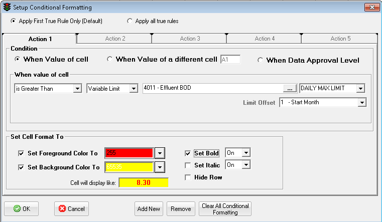
FIELDS:
Apply First True Rule Only (Default): Starting with Action 1 when a condition is met, set the cell format to the Action's format and stop. Example: Action 1 set to Italic if the value >10, Action 2 set to Bold if value > 20. Value of 30 would be Italic because 30 is greater than 10 and the first condition was met.
Apply All True Rules: Starting with Action 1 if a condition is met, set the action and move to the next action. Example: Action 1 set to Italic if the value >10, Action 2 set to Bold if value > 20. Value of 30 would be Bold, Italic.
When Value of Cell: Used to set the cell format based on the value in the cell be formatted. Example: When A1 is greater than 10 set A1 to Bold.
Comparison: Select what type of comparison to make. NOTE: when comparing a text cell the comparsion is NOT case-senstive (i.e. Hello is equal to HELLO, heLLo...). When comparing numeric values, we compare the displayed value to the entered limit (i.e. a cell has a formula of =3.14159 but is displayed to 2 decimals so 3.14 is displayed, 3.14 is compared to the limit NOT 3.14159). Cell when comparing values with data qualifiers the entered value rule is used (i.e. <2 is treated as a 2, >1000 as 1000, ND as 0). Cells containing dates are compared as dates. Choose from the following list.
is Equal to
is Not Equal to
is Greater than
is Greater than or Equal to
is Less than
is Less than or Equal to
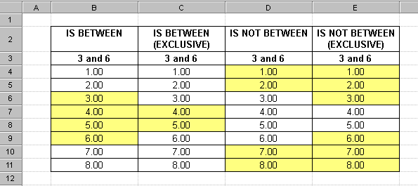
is Between
is Between (Exclusive)
is Not Between
is Not Between (Exclusive)
Contains - If the character(s) entered in the limit are anywhere in the cell.
Does not contain - If the character(s) entered in the limit are NOT anywhere in the cell.
Is Detected - If the cell starts with "ND" or starts with "<".
Is Not Detected - If the cell does NOT start with "ND" or starts with "<".
Is Empty - If the cell is blank or empty.
Compare To: Constant, Cell Value, or Variable Limit.
- Constant: Enter the value to compare to (i.e. 10, Hello)
- Cell Value: You will be prompted to enter a cell reference to get the value to compare to. The cell reference can be an absolute reference ($B$2), or a relative reference (B2).
- Variable Limit: You will be prompted to choose the variable and it's limit (i.e. Daily Max Limit, QC UCL, Entry Min Limit...). Use the Limit Offset to specify the date to get the limit for. For Example, if you are showing three months of daily values (each month is column) and your limit changes every month, for column 2 (2nd month of the report) you would set the offset to 2.
When Value of a different cell: Used to set the cell format based on the value of a different cell. Example: When A1 is greater than 10 set B1 to Bold.
Has the same options as When Value of cell. See above.
When Data Approval Level: Used to set the cell format based on a variables data approval level.
for Variable: Select Variable used for condition
Grouped By: Used with offset, sets which data slot or data range to get the approval level to compare to the Approval Level Specified. The minimum approval level is calculated for the grouping. Example, a grouping of Monthly for a daily variable with an offset of 1 would calculate the minimum data approval of the 31 daily values and compare that minimum to the value specified in the Approval Level. If a grouping of Daily is used with a Daily variable with an offset of 7 the data approval for the variable of the 7th day of the report would be compared to the specified Approval Level.
Offset: Sets the number of ‘intervals' from the start date of the report. Increment by 1, for example, increases the offset by one for the grouping in the Grouped By Field.
is: Select Operator Use operator to specify which data is to be used for the condition
Approval Level: Sets the approval level to use to calculate condition on report.
See Examples 6 and 7.
Set Cell Format To:
Set Foreground Color to: Displays selected color of cell foreground if condition is met
Set Background Color to: Displays selected color of cell background if condition is met
Set Bold: Bolds data in cell if condition is met
Set Italic: Italicizes data in cell if condition is met
Hide Row: Hides the entire row if condition is met.
Cell Will Display Like: Shows what cell will display if condition is met
BUTTONS:
 |
Applies changes and closes form |
 |
Closes form |
 |
Creates a new condition. Conditions are tested in order and once a condition is met the cell if formatted and no other conditions are processed. For example, if you want the cell to be yellow if it is greater than 10, and red if greater than 20 the first action (tab) should check for greater than 20, second tab should check for greater than 10. |
 |
Deletes the current Action for the conditional formatting. |
 |
Removes all condtional formatting from the cells. |
EXAMPLES:
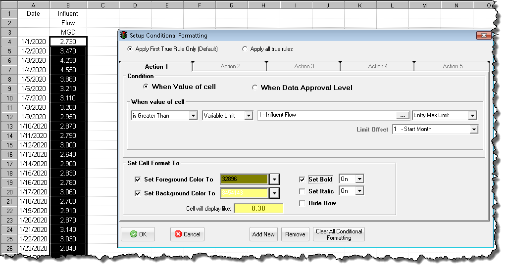
EXAMPLE 1. Set all Influent Flows that are greater than the Entry Max Limit to Bold, green on lite yellow:
1. Locate Influent Flow in spread design using Locate, Daily Values. Placing date beside data and default heading info.
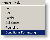
2. Select cell range to format then use Format, Conditional Formatting to set condition for data (Entry Max = 4 in this example)
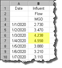
Data that meets condition (Data greater than Entry Limit of 4 for Influent Flow) will now be displayed as follows:
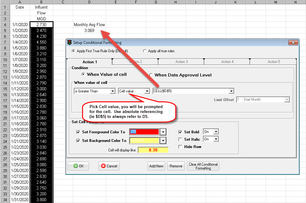
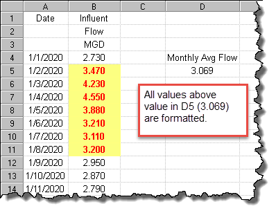
Example 2: Set all Influent Flows that is greater than the Influent Flow Monthly Average Limit to Bold, yellow on red:
1. Highlight cell range and set limit to CELL($D$5). The CELL(XX) command allows you to compare the current cell to a value in a different cell. Use the $ to refer to the cell with absolute referencing, i.e. CELL($D$5) will refer to cell D5 for the entire cell range. CELL(C3) will refer to cell C3, then C4, etc...
Example 3: Using IS BETWEEN
When using Is Between, Is not Between, etc... you specify the range with a dash between the values:
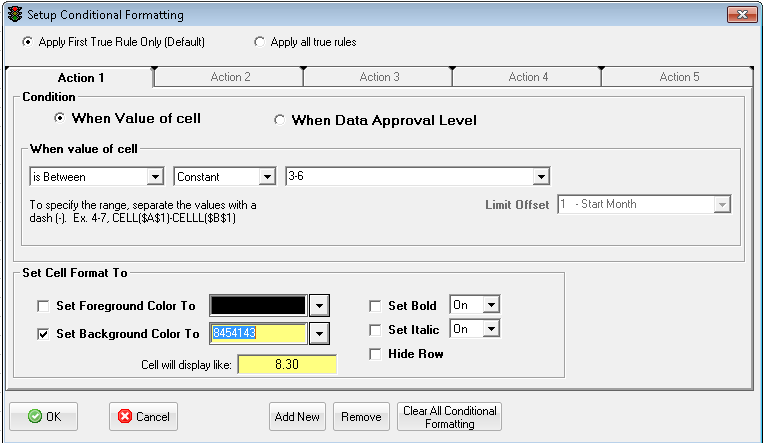
If referring to Cells use Cell(B2)-Cell(B3). Is Between is Inclusive meaning that a value of 3 is considered to be between 3 and 6. Examples
NOTE: If you would like to input negative numbers they will need to be in (). EX: (10)-10 is Negative 10 through 10. The smaller number must be first. EX: (20)-(10) Negative 20 through Negative 10.
Example 4: Setting format based on a different cells value.
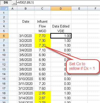
Set a cell to yellow if the data has been edited. We use the VDE function in column D to see if the data is edited. To format column C, we choose When Value of a different cell and set the cell to D6. Note the first cell we are formatting is C6, and since we didn't use absolute references (i.e. $D$6) we will compare look at D6 to format C6, look at D7 to format C7, etc... The VDE function returns a 1 (meaning the data has been edited) so we say when D6 equals 1 set the format. 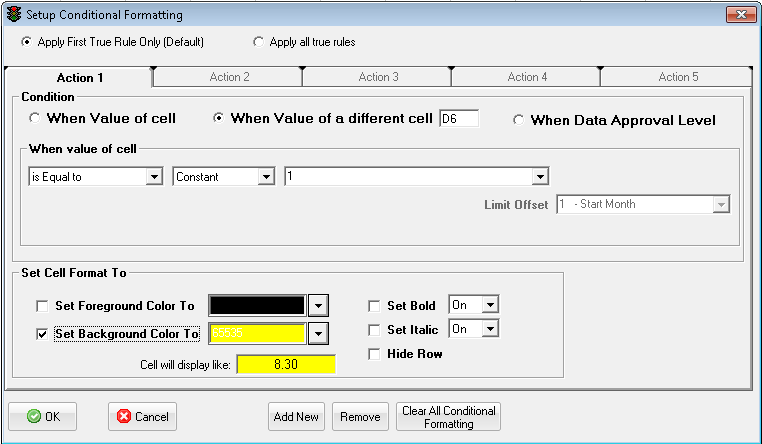
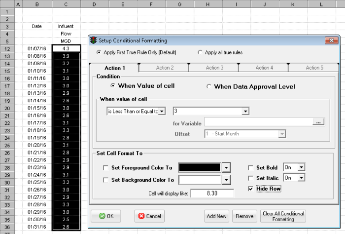
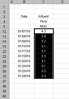
Example 5: Only show days with Flows greater than 3 using Hide Row:
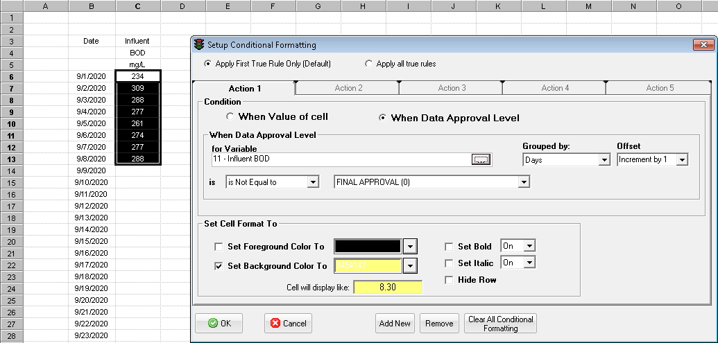
Example 6: Set background to yellow for Influent BOD unapproved data
Since Influent BOD is a daily variable and I want to compare each day's data approval level I use a grouping of Days with an Offset of Increment By 1. This means the first cell in the block (C6) will find the data approval level for the 1st day of the report and check if it is not equal to FINAL APPROVAL. Cell C7 will find the data approval level will use an offset of 2 and find the data approval level for the 2nd day of the report.
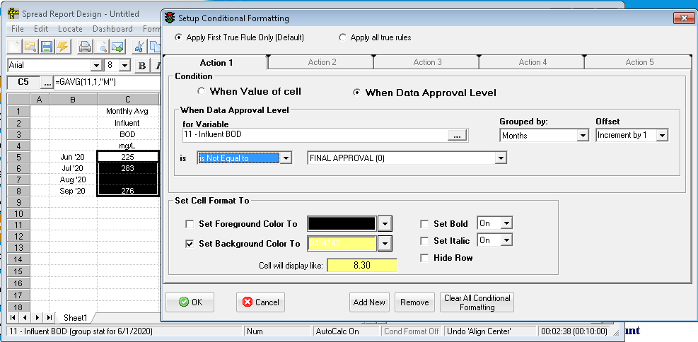
Example 7: Set background to yellow for any month that has an unapproved Influent BOD
Group by Months. For cell C5, the minimum Data Approval level for Influent BOD for June 2020 (1st month of the report) will be calculated and if it is not equal to FINAL APPROVAL the cell will be set to yellow. For cell C6, the minimum Data Approval Level for July 2020 (2nd month of report) will be compared.
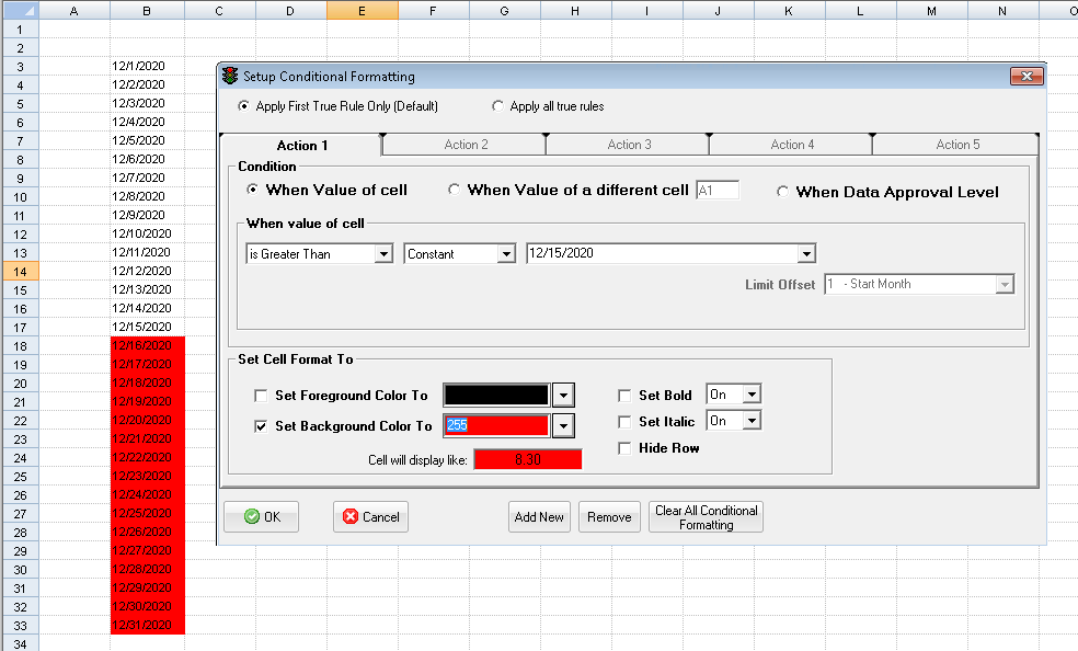
Example 8: Set background to red for all dates greater that 12/15/2020
NOTE: If a cell contains a date, time, or a date/time it is compared as a datetime not as a string.
NOTES:
The following tables explain how comparisons are performed.
| Cell Value |
Limit |
Is Greater (>) |
Is Equal (=) |
Is Less Than (<) |
Contains |
| 3.14159 (shown to 2 decimals) |
3.14 |
False |
True |
False |
False |
| Apple |
B |
False |
False |
True |
False |
| Apple |
APPLE |
False |
True |
False |
True |
| Cell Value |
Limit |
Is Greater (>) |
Is Equal (=) |
Is Less Than (<) |
| <2 (will be treated as 2) |
2 |
False |
True |
False |
| >100 (will be treated as 100) |
100 |
False |
True |
False |
| ND (will be treated as 0) |
2 |
False |
False |
True |
| Cell Value |
Is Detected |
Is Not Detected |
Is Empty |
| 45 |
True |
False |
False |
| <2 |
False |
True |
False |
| 0 |
True |
False |
False |
| >100 |
True |
False |
False |
| "" - Blank cell |
False |
False |
True |
| ND |
False |
True |
False |