Continuing from Lab 2.2.3, we will improve the look of the Monthly BOD/TSS report.

1. Set the font of the title.

Click on cell E2.
Select Format, Font. 
Select any font and size you like and click OK.  The title will be changed to the font specified.  Notice the whole title changed not just the text in the cell. 

 

2. Add titles at the top of each column. 

Move to Cell B6 and type “Date”.
Enter the other titles as shown in the figure below.

3. Draw Borders. Borders are lines drawn on the outside of cells.  They can be used to break up a report into logical sections making the report more readable.  The grid (the light gray lines you see on the spreadsheet) is not printed and is on the screen to make the spreadsheet easier to navigate. 

Highlight Cells B5 through G6 (B5:G6).  To select a block of cells, click on a cell while the cursor is in the cell selection mode   , hold the mouse button down and drag the mouse to select multiple cells (selected cells appear in black).  Once a block of cells is selected, you can change the font, border, color, etc. of all selected cells with a single command.

To set the border, Select Format, Border with the cells highlighted.

Select Box Columns as shown below and click OK.

 

 
Now, set the following borders.

Cells: D5:E5
Border: Outline Selected Cells

Cells: F5:G5
Border: Outline Selected Cells

Cells B7:G40
Border: Box Columns

  

4. To resize a column, move the mouse pointer between the columns as shown in the Figure below.  The mouse pointer will change and you can then drag the mouse left to shrink the column or right to enlarge the column.  To adjust the row height, move the mouse pointer between the row's headers.  The mouse pointer will change and you can then drag the mouse (by clicking and holding the button) down to enlarge the row or up to shrink the row.
 

TIP: To resize multiple columns at one time, select all the columns by clicking and dragging the mouse on the column headers.  With the columns selected, resize one of the selected columns and all the selected columns will be sized the same.  This method can also be used to resize multiple rows at one time.  See Resizing Columns and Rows in Spread Reports Design video in help system to learn more tips and tricks on resizing.

5: Improving your report:

Let’s add a new column to your report. 
1. Using the mouse, select cell F7. 
2. Click on Edit, Insert column. 
3. Column F should now be blank.
4. Highlight cells G5:H40.  Move the mouse pointer to the edge of the selected columns until the pointer shows an arrow.

 

5. Click and hold the mouse button to drag the selected columns one space to the right.
 
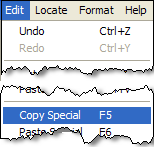
6. Select cells D5:E6.  Select Edit, Copy Special (or press F5) 

7. Move to F5 and press Edit, Paste Special (or press F6). Label cell F5 “Primary Effluent”.  
 

7. Now, locate your new variables just as in Step 2.
 
Cells: F7-F40
Variable: 611 - PriEffBOD
Cells: G7-G40
Variable: 613 – PriEffTSS
 
 

At this point you can use the border formatting to box the newly added columns.  Also, for review, locate the Monthly Summary Average and Maximum for the Primary Clarifiers.  Save the report.  You have now created your first spread report.  You can use the tools you have learned in this section to create as many custom reports as you wish in a variety of different formats.  This may be a good time to take a break, or move on to the next section.

Next>